Hi.
The pre-processing I had in mind, and I was mentioning in my previous post, would happen outside PV, namely in Python. I am completely lost when it comes to code inside the PV env., and I cannot help you with that. So, in Python, I would manipulate my dataset so to “bake” it in a way and shape that PV likes it. I would go for netCDF format which is cross-platform, and contains all the metadata you might need, for possible future inspections.
Conceptually:
the wave model I am working with, spits out one single matlab binary file that contains all variables for all timesteps. In this example, it includes flow velocity varying over time and space:
Velmag_k15_000001_200
would mean:
quantity Velmag (velocity magnitude)
k15: layer number 15 (with k in range[0, k_bottom]; k=0 is the actual free surface)
000001_200: time here equals 1.2 seconds (format is HHMMss_mms)
In my simple1D case, I merge all layers into one matrix having Nr_of_Layers rows and Nr_of_x_gridpts columns. I repeat that, recursively, for all timesteps. The result is converted to a netcdf files (Python, xarray), saved on disk, and ingested in PV.
For depth-averaged flows, if you want to (fictitiously) recreate a filled contour effect, you need to create a matrix like the one I have described above, with only two lines. The content of these liens is the value of, for instance, flow velocity (or pressure, or momentum, or whatever) and:
- to the first row, you assign z coordinates of the free surface
- to the second row, you assign z coordinates of your bathymetry.
I am trying to achieve exactly that in Python now. However, the problem I am facing is that the topology of my z coordinates changes over time. And PV seems to be unable to understand that.
If you have a time-invariant z coordinate topology, your problem is very easy to solve.
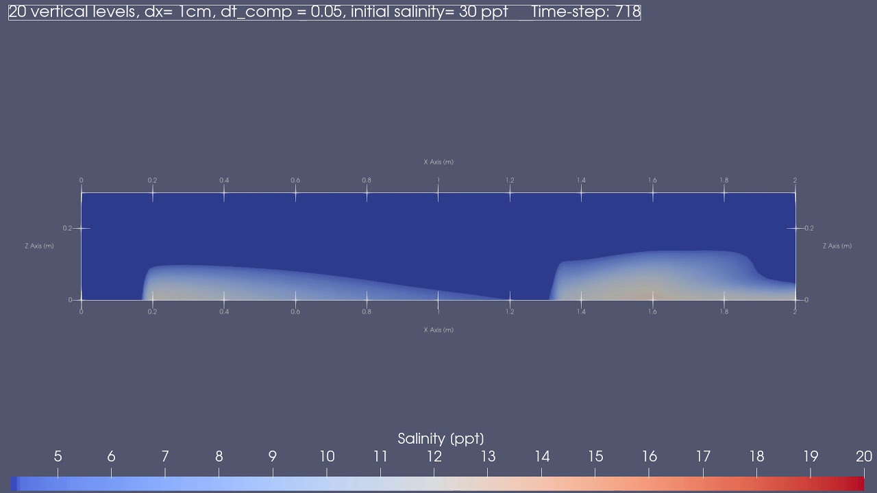
So far, I could achieve something like this:
If you want, send me two or more time-steps PLUS bathymetry of your model results and I can code it for you as an example.
Should be pretty straightforward.
Ciao.
