Placing Objects on Terrain - PALM NetCDF Files

[patrickzerhusen (Patrick)]

Helo together,

I tried to visualize PALM NetCDF simulation results (_3d.000.nc) and a PALM NetCDF static driver (objects in model domain) (_static.nc) in ParaView.

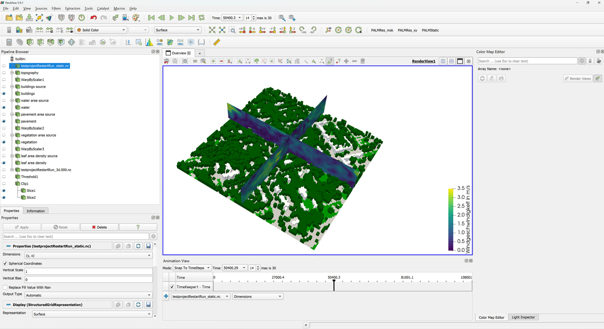
I displayed the static driver using a threshold filter for buildings_3d (dimensions: z, y, x; minimum: 1, maximum: 1), water_type, pavement_type, vegetation_type (dimensions y, x; minimum: 0, maximum: 15) and lad (dimensions: zlad, y, x; minimum: 1, maximum: 1).

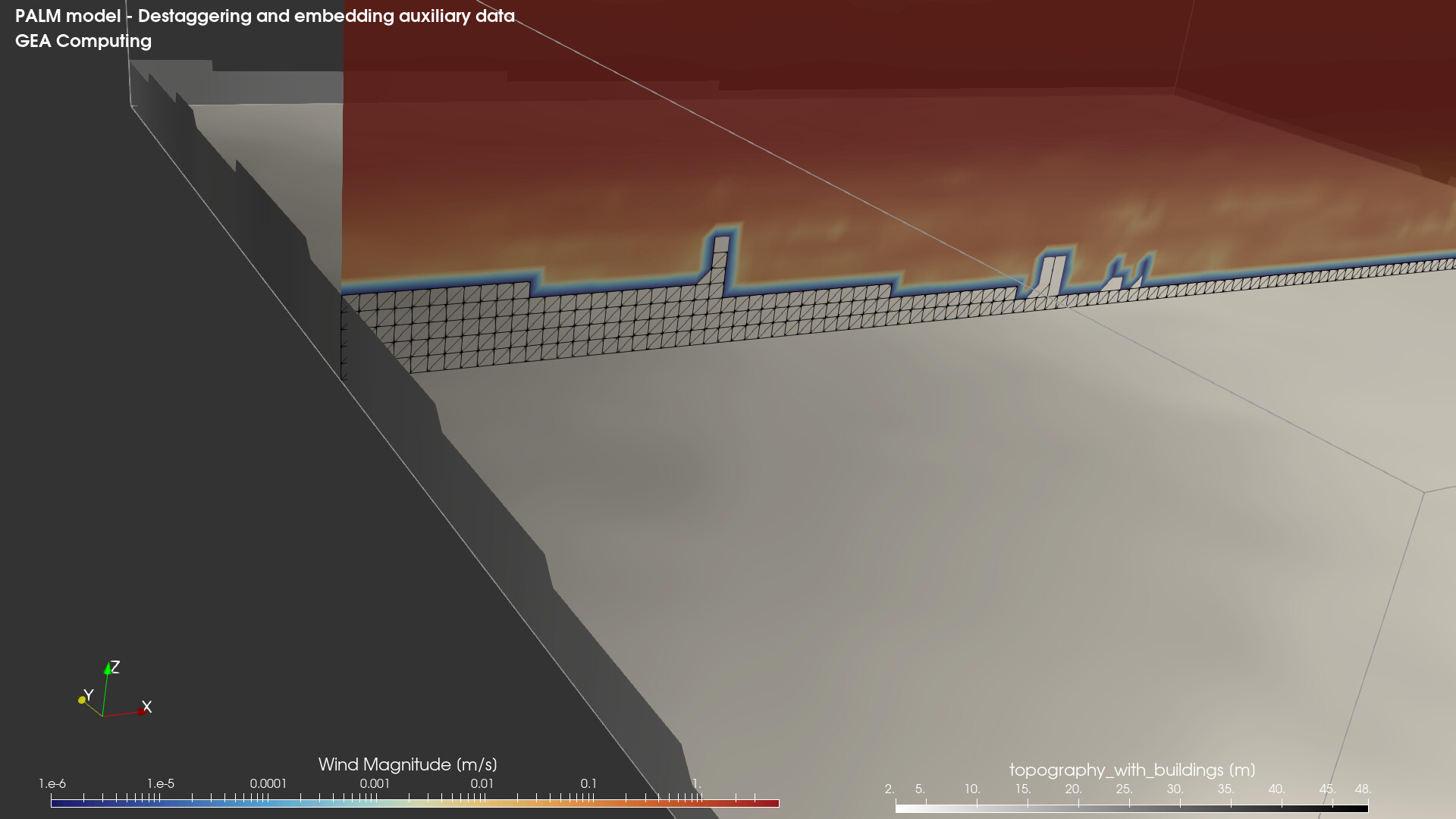
I displayed the simulaiton results (dimensions: zu, y, x; representation: surface; coloring: wspeed) using a threshold filter (minimum: 0, maximum: 99999 to remove NaNs), a clip filter (clip type: box; invert), and slice filters (slice type: plane).

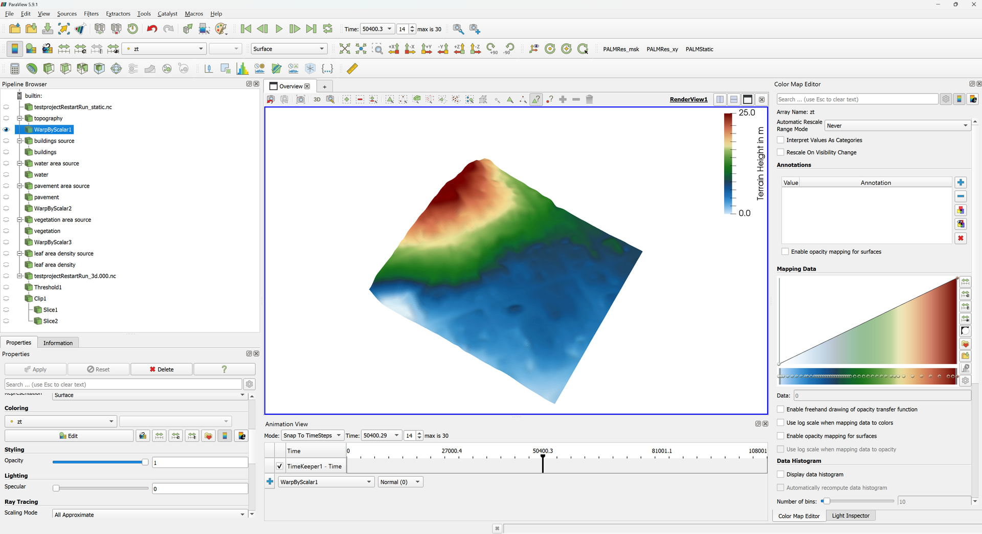
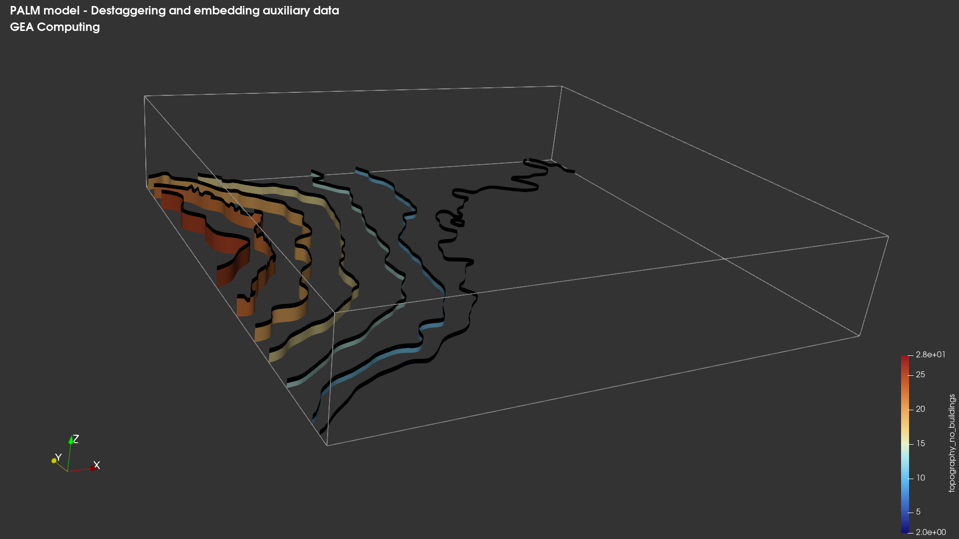
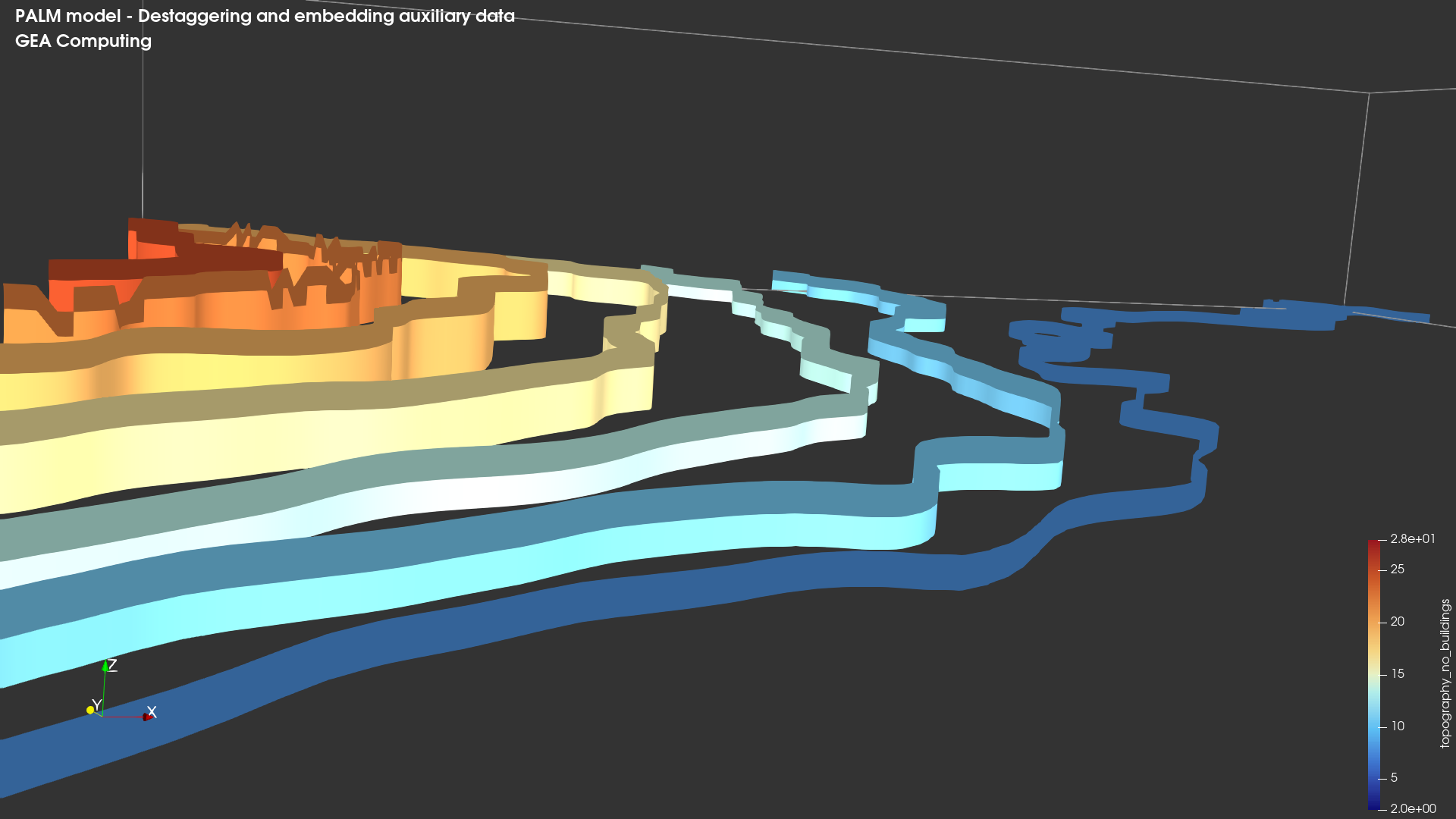
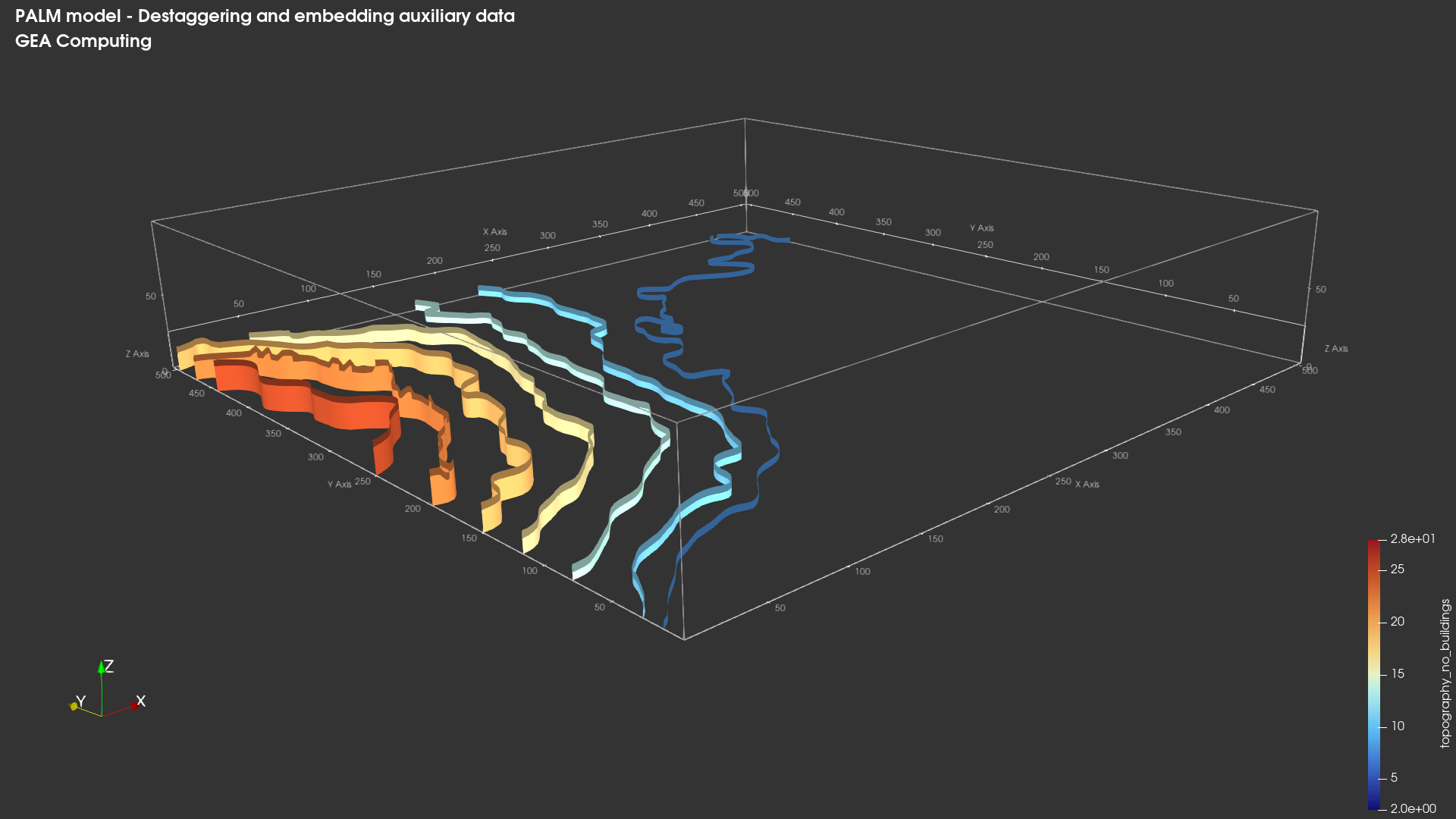
The topography (dimensions: y, x; coloring: zt) was displayed using a warp by scalar filter (scalars: zt; scale factor: 5)

Of course, like this, the static driver and simulation results remain on a flat plane while the topography projects above it.

I think, water_type, pavement_type, vegetation_type could be processed with the warp by scalar filter. But how can I place buildings_3d and lad onto the 3D topography?

Could I use filters in ParaView or should I preprocess the NetCDF files in Python? I would prefer a ParaView-based solution, but if that is not feasible, a Python-based approach is also acceptable.

I understand that probably few people have experience with PALM NetCDF files, so let me know what other information you need!

[geacomputing (GEA Computing Ltd.)]

Hi there @patrickzerhusen

interesting question you’re posing here.
Is there any change you could share (a sample of) your data, here? I’d like to give it a little quick try.

Also are u and v staggered? If so, have you unstaggered them (already)?

Cheers

[patrickzerhusen (Patrick)]

Hi @geacomputing,

thanks for reaching out! Sorry for the delayed response - I was on vacation. I will send you the sample dataset I used to take the screenshots.

I’d really appreciate your feedback!

Kind regards,

Patrick

[geacomputing (GEA Computing Ltd.)]

Hi there, Patrick.

Thanks for the data.

I played around a bit and, based on what you have, my advice would be NOT to use PV’s in-built filters. Instead, I would preprocess using Python (e.g., xarrary!). Some processing steps, especially grid unstaggering, are much more agile in python than they are in PV. Once happy, you can then export to netcdf or vtk (both work!).

What I did was:

1. de-staggering the grid (natively Arakawa staggering), so that everything falls on a common playground. Based on my experience, this is the best way to go when “merely” visualizing data.
2. Adding (re-broadcasting) topography on the same, newly destaggered, grid. This eliminates the tedious need of playing with extrusion factors and scaling. The model generates the output, both prognostic and static, and, without ever have to rescale, you use them 1 to 1.

The result is a consistent, all contained, de-staggered dataset where buildings end up “sitting” on topography. For this exercise I have created and appended two topographies, one with and one without buildings. When plotting it, everything is consistent. What works for buildings, can work just as fine for other variables (leaf coverage, soil moisture, etc…).

For destaggering, in xarray, for u component:

u_vals = 0.5 * (
sim[“u”].isel(xu=slice(0, -1)).data
+ sim[“u”].isel(xu=slice(1, None)).data
)

u = xr.DataArray(
u_vals,
dims=(“time”, “zu_3d”, “y”, “x”),
coords={
“time”: sim.time,
“zu_3d”: sim.zu_3d,
“y”: sim.y,
“x”: sim.x.isel(x=slice(0, u_vals.shape[-1])),
},
name=“u”,
)

Then re-broadcasting topography:

#--------------------------------------------------
#Topography and buildings volumes
#
#
#topography_no_buildings(zu_3d, y, x):
# = zt where zu_3d <= zt
# = NaN elsewhere
#
#
#topography_with_buildings(zu_3d, y, x):
# = zt where zu_3d <= zt
# = zt + buildings_2d where zt < zu_3d <= zt + buildings_2d
# = NaN elsewhere
--------------------------------------------------

base3d = out[“theta”].isel(time=0, drop=True)
zcoord = base3d[“zu_3d”]

zt2d = static[“zt”].isel(
y=slice(0, ny),
x=slice(0, nx),
).assign_coords(
y=common_y,
x=common_x,
)

bld2d = static[“buildings_2d”].isel(
y=slice(0, ny),
x=slice(0, nx),
).assign_coords(
y=common_y,
x=common_x,
)

zt3d = zt2d.broadcast_like(base3d)
bld3d = bld2d.broadcast_like(base3d)

building_top = zt3d + bld3d

Terrain only

topography_no_buildings = zt3d.where(zcoord <= zt3d)

This is, I believe, the most efficient approach especially if you are interested in showing for example flow around buildings or terrain. Of course, the higher the model resolution, the better the buildings will be resolved (and thus the nicest the results will be).

Hope this helps.