How can I use 2D data (x coordinate, y coordinate, z coordinate-bottom, water elevation z coordinate-top, x velocity, y velocity) to create a visualization for top water surface along with the side walls and bottom surface of the river channel in paraview? Any help will be very much appreciated.
Hi @nsh , you should be able to use the “Warp Scalar” to produce a 3D mesh from your 2D data. You can apply it once to the reader’s output to obtain the river bottom surface and a second time to the reader’s output to get the water’s top surface. Then color the water top surface by the velocity vector you have.
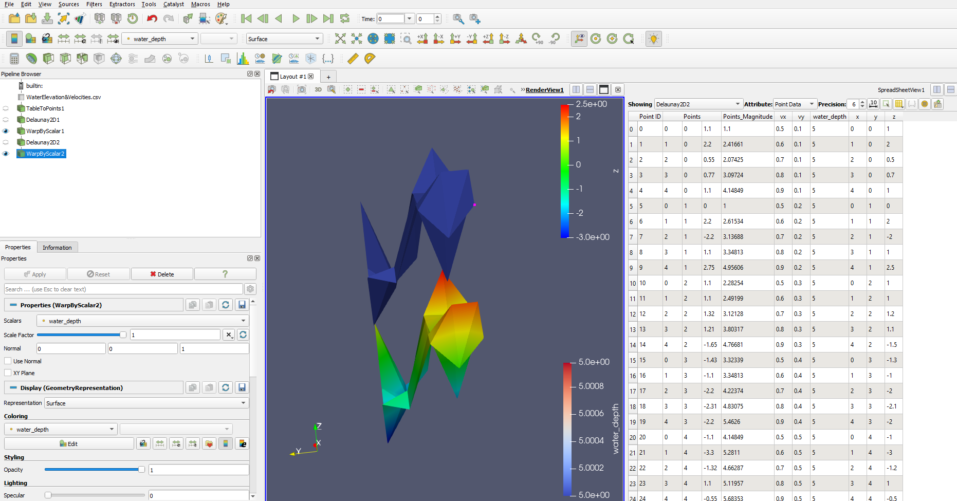
@nsh It looks like the water_depth is 5.0 for all of the input points, so that would be expected; the two surfaces are separated by a distance of 5.
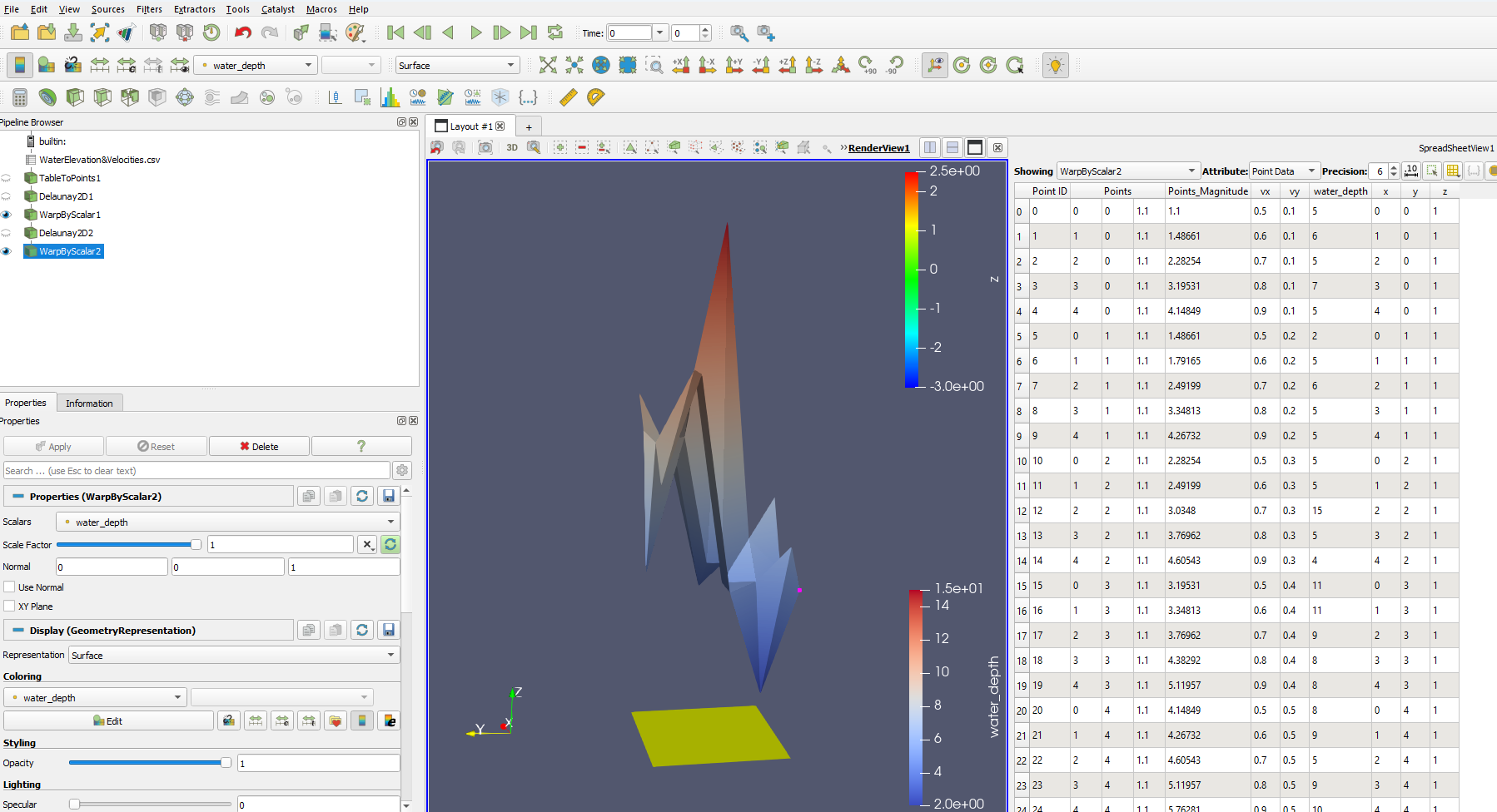
Hi David: I understand and agree with what you are saying. I fixed the bottom surface and replotted the top surface using warp vector. It is now behaving as expected. I have already plotted the bottom surface of the river bed. What’s the best way to plot the side walls of the river channel. Any thoughts?
@nsh In the attached state file, I’ve used (1) a FeatureEdges filter, (2) a Ribbon filter, and (3) a Calculator to create a “cap” for the space between two WarpScalar filters.
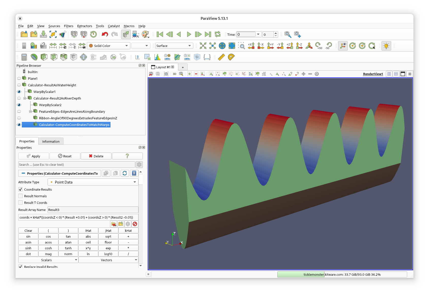
The first two Calculators compute sine waves on a PlaneSource to simulate the water height and riverbed depth (both measured from a “mean sea level” of 0.0). Then the WarpScalars produce the top (colored by Result) and bottom (colored brown) surfaces.
Then, the 3 filters mentioned up top (1) compute the boundary edges of the input surface; (2) extrude the boundary edge up and down, above and below the z=0 plane where the input surface – not the warped surfaces – lies; and (3) warp the ribbon surface to match the top WarpScalars on one edge and bottom WarpScalars on the other.
The final Calculator replaces the input Ribbon filter’s coordinates with warped versions:
coords + kHat*((coordsZ > 0) * (Result - 0.01) + (coordsZ < 0) * (Result2 + 0.01))
coords are the input point coordinates (vectors) and kHat is a unit vector in the Z direction.
One edge of the ribbon (where coordsZ > 0 ) is warped by “Result - 0.01” and the other edge of the ribbon (where coordsZ < 0 ) is warped by “Result2 + 0.01”. The “0.01” values in the formula must match the Width property of the Ribbon filter. Note that (coordsZ > 0) is 1 on the top edge of the ribbon and 0 on the bottom edge. Similarly (coordsZ < 0) is 1 on the bottom edge of the ribbon and 0 on the top edge.
Hi NH.
In the past, I have worked too with model data following the same structure you describe, that is:
-topology or coordinates (x,y,z) and
-(multiple) scalar field(s), such as temperature, pressure or velocity components.
What I did to visualize it was described in a few blog post in the forum (see links below), to recreate large scale scenarios for my atmospheric model (WRF). As an example, I have demonstrated how the same applies for ocean model (ROMS), where Z axis is pointing down (below water).
You can either work directly with netcdf (model output) or, if you need custom manipulation and reprocessing, you can generate your own vtk (I did that in python).
The blog posts have some code included. I hope you will find it interesting. The links are:
Also, there are some video on YouTube I created some 5 years ago showing just that. Just search for "swash wave model paraview). This is one example:

Hope this helps.